Fluorescence Lifetime Imaging Microscopy (FLIM) has emerged as a powerful technique for quantitative imaging in biological research. By measuring the fluorescence decay time of excited molecules, FLIM provides critical insights into the cellular environment, molecular interactions, concentration, and dynamic processes. This application note describes the implementation of feedback microscopy using FLIM data, focusing on the versatility and ease-of-use of NIS-Elements software and the Nikon AX R Confocal Microscope, combined with the PicoQuant FLIM Addon.
Introduction
FLIM is a powerful imaging method that measures the time it takes for a fluorophore to return to its ground state after excitation. This technique offers several advantages over traditional intensity-based fluorescence measurement. Unlike intensity-based measurements, fluorescence lifetime is independent of fluorophore concentration, photobleaching, and other variations, offering a robust parameter for various cellular studies [1]. Combining this powerful lifetime data set together with feedback microscopy would provide effective screening of a cell population. Indeed, feedback microscopy integrates real-time data analysis to make decisions upon analysis results and guide subsequent imaging or photomanipulation tasks. In this application note, we challenge feedback microscopy based on intensity measurements over the fluorescence lifetime parameter for robust, sensitive and environment sensitive applications. Fluctuation of fluorescence lifetime of a cell population was recorded over time and used to further identify a subset of cells exhibiting the largest variation in fluorescence lifetime. These identified cells can be selected for automatic photo-stimulation or other microscopic tasks. This workflow is enabled by the seamless integration of Nikon AX R Series Confocal Microscope (here after AX R) with PicoQuant FLIM LSM Upgrade Kit (here after PQ RapidFLIM) for images acquisition, and NIS-Elements software (here after NIS-E) for analysis.

Keywords: Confocal, FLIM, Feedback Microscopy, time-lapse, calcium signaling, live cell imaging, SMART microscopy
Result
One of the advantages of calcium variation studies using lifetime measurements is to avoid potential saturation of the calcium dye that intensity ratio measurements could be prone to, therefore leading to considerable errors when measuring calcium concentration. In addition, FLIM avoids such limitations by using a specific calcium sensor (e.g. expressing a large dynamic range to detect large variations of fluorescence intensity) and it makes the use of calcium dyes in the UV range obsolete.
Madin-Darby canine kidney (MDCK) strain II cells were loaded with Oregon Green-BAPTA 1 (OGB1) for 30 minutes at room temperature and subsequently imaged using the A-1 R with EQ rapidFLIM (Photon counting Hybrid detector and MultiHarp150) and 40 MHz pulsed laser excitation at 485 nm. A continuous timelapse acquisition was recorded for 3 minutes and 3 images of arriving photons were integrated for each acquisition timepoint. Lifetime changes were visualized using Time-correlated Single Photon Counting electronics (TCSPC).
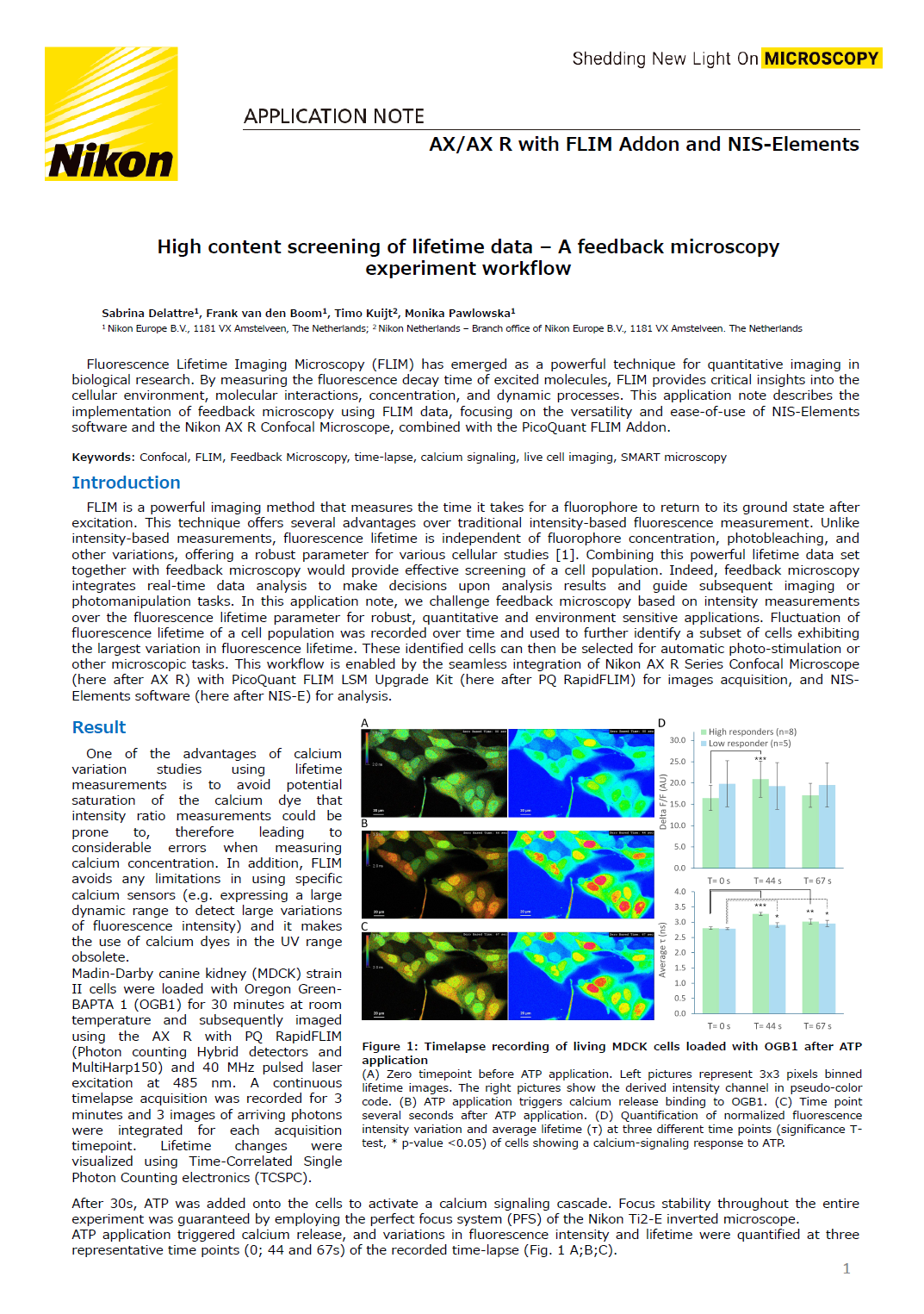
After 30s, ATP was added onto the cells to activate a calcium signaling cascade. Focus stability throughout the entire experiment was guaranteed by employing the perfect focus system (PFS) of the Nikon Ti2-E inverted microscope. ATP application triggered calcium release, and variations in fluorescence intensity and lifetime were quantified at three representative time points (0; 44 and 67s) of the recorded timelapse (Fig. 1 A;B;C).
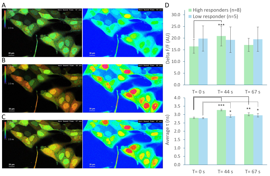
Figure 1: Timelapse recording of living MDCK cells loaded with OGB1 after ATP application.
(A) Zero timepoint before ATP application. Left pictures represent 3x3 pixels binned lifetime images. The right pictures show the derived intensity channel in pseudo-color code. (B) ATP application triggers calcium release binding to OGB1. (C) Time point several seconds after ATP application. (D) Quantification of normalized fluorescence intensity variation and average lifetime (τ) at three different time points (significance T-test, * p-value <0.05) of cells showing a calcium-signaling response to ATP.
Significant calcium release of individual cells was observed after approximately 40s, revealing two distinct cell responses. The first group, referred to as "High responders", exhibited the largest changes in fluorescence intensity, indicated by a significant release of calcium 44s after ATP stimulation. In contrast, the second population showed no detectable variation in fluorescence intensity (Fig. 1D).
The same population was then analyzed using FLIM data. High responders displayed a lifetime shift from 2.8ns ± 0.05 at 0s to 3.3ns ± 0.05 following ATP application (44s) which remains significant at 67s (Fig. 1D). Interestingly, while no change in fluorescence intensity was observed in the second population, a significant increase in the lifetime was observed at both 44s and 67s time points. Note the smaller standard deviation of the FLIM data compared to fluorescence intensity-based measurements. This observation aligned with Agronskaia et al [2], who reported that OGB1 lifetime ranges from 2.5ns to 3.7ns depending on the calcium concentration.
This straightforward experiment illustrates that FLIM offers a more robust measure as opposed to intensity-based parameter, allowing more reliable quantification. The change in lifetime depicted in Fig. 1D can be observed in real time using the phasor plots representation (Fig. 2B). The phasor plot is a graphical representation of raw FLIM data in a vector space. One pixel of a FLIM image represents one point in the phasor plot. In case of single decay component (mono-exponential) the lifetime is located on the universal phasor plot arc. In contrast, a multi component lifetime is positioned inside the universal arc.
Figure 2: Phasor plot representation of the lifetime shift of OGB1 upon ATP application (A) An alternative representation of lifetime at three different time points (timepoint: T=0; T=44s; T=67s, upper, middle, bottom image respectively). All pixels with an average lifetime > 2.25ns are displayed in green, all pixels below 2.5ns are displayed in red. (B) Phasor plot representation of the average lifetime of the entire frame. Note the shift in lifetime during ATP application (middle).
We next sought to investigate whether FLIM data could be effectively integrated into a SMART experimental protocol. The aim is to automatically identify and select a population of cells with a distinct response and target individual cells for subsequent advanced acquisition or analysis (Fig. 3A).
As proof-of-concept we decided to focus on the cells with the highest calcium response. We envisioned this population could potentially be relevant for assessing drug response kinetics and/or understanding whether early responding cells may trigger neighboring cells responses.
We developed a General Analysis 3 (GA3) analysis workflow where segmentation of individual cells was performed on fluorescent intensity extracted from average lifetime data (Fig 3A and B).
Segmenting closely adjacent cells can be a complex and challenging task, particularly when selection of cells is based on average lifetime measurements and when images have low resolution. Thus, segmentation was assisted by using an AI tool (SegmentObjects.ai), which was pre-trained before the experiment on intensity-based data. SegmentObjects.ai segmented objects faster than intensity thresholding and more accurately, even on images with large pixel sizes (data not shown). Therefore, AI segmentation tools provide a strong advantage in experiments that focus on fast dynamic studies rather than highly resolved images.
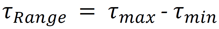
A key concept for SMART image acquisition is to automate the workflow and aim for minimal user-based interaction when the experiment is progressing (Fig. 3A). Therefore, the first step of the automatic SMART imaging acquisition was to compute the average lifetime (τ) of all cells as a population average. Then we calculated the lifetime change over time per segmented object (individual cell) by normalizing τ over the average lifetime range of the whole population (Fig. 3C) using the following equation :
We calculated the Standard Deviation of τRange (StDev τRange) and Mean τRange. By calculating these two parameters we gained knowledge on the overall lifetime responses of the population and thus can select the High responders without prior knowledge of the population response by using dynamic thresholding strategy. We introduced a multiplication factor to adjust StDev τRange weight on the dynamic threshold equation as followed :

Our GA3 protocol compiles different outputs such as: objects parameters (cell ID, size, coordinates, Norm τ, etc...), binary masks (Fig. 3B) and lifetime change over time plots (Fig. 3C) enabling tracking of objects of interests (in our example the High responders). The only user-inputs required are specified before automated image acquisition process begins. The required inputs are 1) the τ threshold and 2) the number of cells to be imaged (e.g., 1000) for statistically significant data set. This fully automated SMART microscopy acquisition allows (re)-imaging and/or analyzes solely on the required cells. This feedback loop continues until the target is reached.
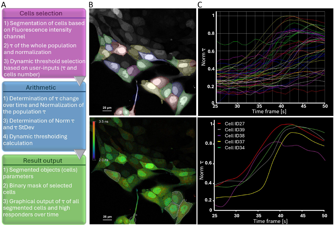
Figure 3: Dynamic threshold application for High responder selection (A) Schematic explanation of JOBS/GA3 recipe created within NIS-E using pre-trained ai network (SegmentObject.ai). (B) Segmentation based on intensity of all cells (top). High responder cells selected based on the strongest variation in fluorescence lifetime (bottom). (C) Plotted Norm τ of all segmented cells (top) and High responders (bottom) over time.
Conclusion and Outlook
In this application note, we created an experimental workflow that showcases the Nikon AX R - PicoQuant FLIM as a versatile and user-friendly solution for high content imaging and screening. The workflow we developed provides a strong foundation on which many user-specific applications can be built from. GA3 enables virtually any parameters to be computed from FLIM data, thus one could envision limitless possibilities for cell selection based on various output parameters. In addition, the created workflow generates binary masks that could easily serve for photoconversion/photoactivation of cells which can be subsequently isolated for downstream analysis. Lastly, the integration of a Python node in NIS-Elements version 6.10 expands these opportunities by offering an import function of acquisition and/or analysis scripts generated outside NIS-Elements, thereby facilitating the integration of pre-existing analysis and/or protocols with other hardware.
Acknowledgment
We would like to express our gratitude to Prof. C. Lohr (Neurophysiology, Inst. Cell and Systems Biology of Animals, University of Hamburg, DE) for providing cells and reagents. In addition, special thanks to Christian Börrchen (Nikon DE Branch) and Fabian Jolmes (PicoQuant GmbH) for their help with image acquisition. Finally, we would like to thank Andrii Rogov (Nikon Europe B. V.) for his support on the JOBS and GA3 protocol.
References
[1] Rupsa Datta, Tiffany M. Heaster, Joe T. Sharick, Amani A. Gillette, Melissa C. Skala, J. Biomed. Opt. 25(7), 071203 (2020), doi: 10.1117/1.JBO.25.7.071203
[2] A. V. Agronskaia et al; Journal of Biomedical Optics 9(6), 1230-1237 (November/December 2004)
Product information
AX/AX R Confocal Series
Nikon AX-R Confocal Microscope: Known for its large 25mm field of view, high resolution and advanced imaging capabilities. PicoQuant FLIM Addon: Provides fast FLIM Electronics (Multiharp150) and pulsed PicoQuant laser sources for precise FLIM measurements.
NIS-Elements Software
Nikon's comprehensive imaging software for data acquisition, analysis, and control including JOBS visual experiment generator and General Analysis 3 (GA3) to create a powerful analysis workflow of fluorescence lifetime data during acquisition.
-
Nikon AX-R
-

Product information is here
스펙